Model Parameter Estimation
05 Apr 2021 - Academia
Dark adaptation models
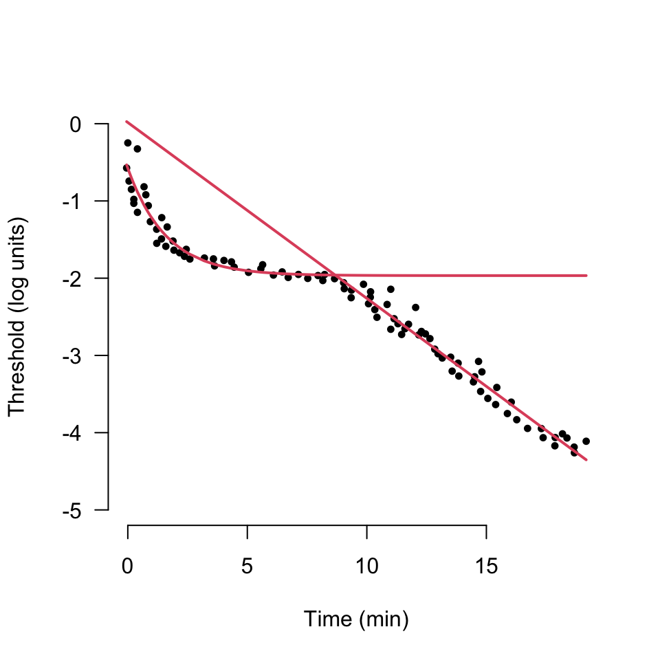
There are at least two models used in the literature. The first is a twin exponential decay

the second, an exponential, bilinear model, is more complex and was first described by Mahroo and Lamb (ref)
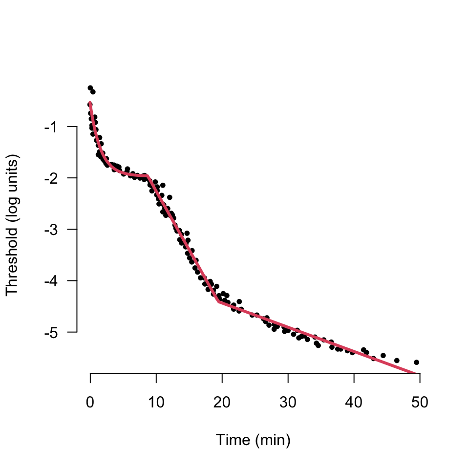
We are concerned with a reduced form of the Mahroo and Lamb Model with only five parameters.The threshold $Thr~(log(cd.m^{-2})$) with respect to $time~(minutes)$ of adaptation is defined as the sum of the Cone response;
where $CT$ is the absolute cone threshold ($log(cd.m^{-2})$), $CC~(log(cd.m^{-2})$) the cone offset at time zero, and the time constant of recovery $\tau~(minutes)$, and the Rod threshold;
where $S2~(log(cd.m^{-2}).min^{-1})$ is the rate limited rod recovery rate, $\alpha~(min)$ is the time when rod sensitivity is greater than cone sensitivity, and $k$ is a dimensionless value. The denominator ensures that rod contribution to sensitivity is nil before $\alpha$ and additive after, the value of $k$ affects the rate of switch transition and is discussed in the appendix.
Hence the estimated threshold for a time $t$ and model parameter estimate $\boldsymbol{\hat\theta}$ is; \begin{equation}\label{eqn:est} \tag{1} Thrs(\boldsymbol{\hat\theta}, t) = \theta_1 + \theta_2\exp\Big({\dfrac{-t}{\theta_3}} \Big) + \theta_4\dfrac{(t-\theta_5)}{1 + \exp{(-k*(t - \theta_5)})}\end{equation}
and it follows that the residuals can be written as a vector $\bf{R}$ where
\begin{align}\label{eqh:resi}
\boldsymbol{R(\hat\theta)} &= \begin{bmatrix}
thrs_1 - Thrs(\boldsymbol{\hat\theta}, time_1) \cr
thrs_2 - Thrs(\boldsymbol{\hat\theta}, time_2) \cr
thrs_3 - Thrs(\boldsymbol{\hat\theta}, time_3) \cr
\vdots
thrs_n - Thrs(\boldsymbol{\hat\theta}, time_n)
\end{bmatrix}
\end{align}
Finding the parameters
We are interested in the parameters ($\boldsymbol{\theta}$) of the model described above, a common technique takes a number ($n$) of threshold measurements over time and calculates the difference between the actual measurements and estimated values for a given set of parameters. These differences are squared and summed, then the parameters of the model are modified until the sum of squares is at a minimum, the final parameter values are then considered optimal. The sum of the squared differences of the measured threshold and the estimated threshold is minimised, such that when $L(\boldsymbol{\theta})$ is at a minimum, the values of $\theta$ are the best estimate.
This objective function can be written using $\odot$ to express element wise multiplication \(L(\boldsymbol{\hat\theta}) = \sum_{i = 1}^{n}{\boldsymbol{R(\hat\theta)}\odot \boldsymbol{R(\hat\theta)}}.\) We use element wise multiplication notation to retain the $\sum$ notation.
When $L(\boldsymbol{\hat\theta})$ is at a minimum, $\dfrac{dL}{d\boldsymbol\theta} = 0$. We can use the gradient of the slope of the objective function to locate the minimum of the function using a gradient descent method.
Gradient descent
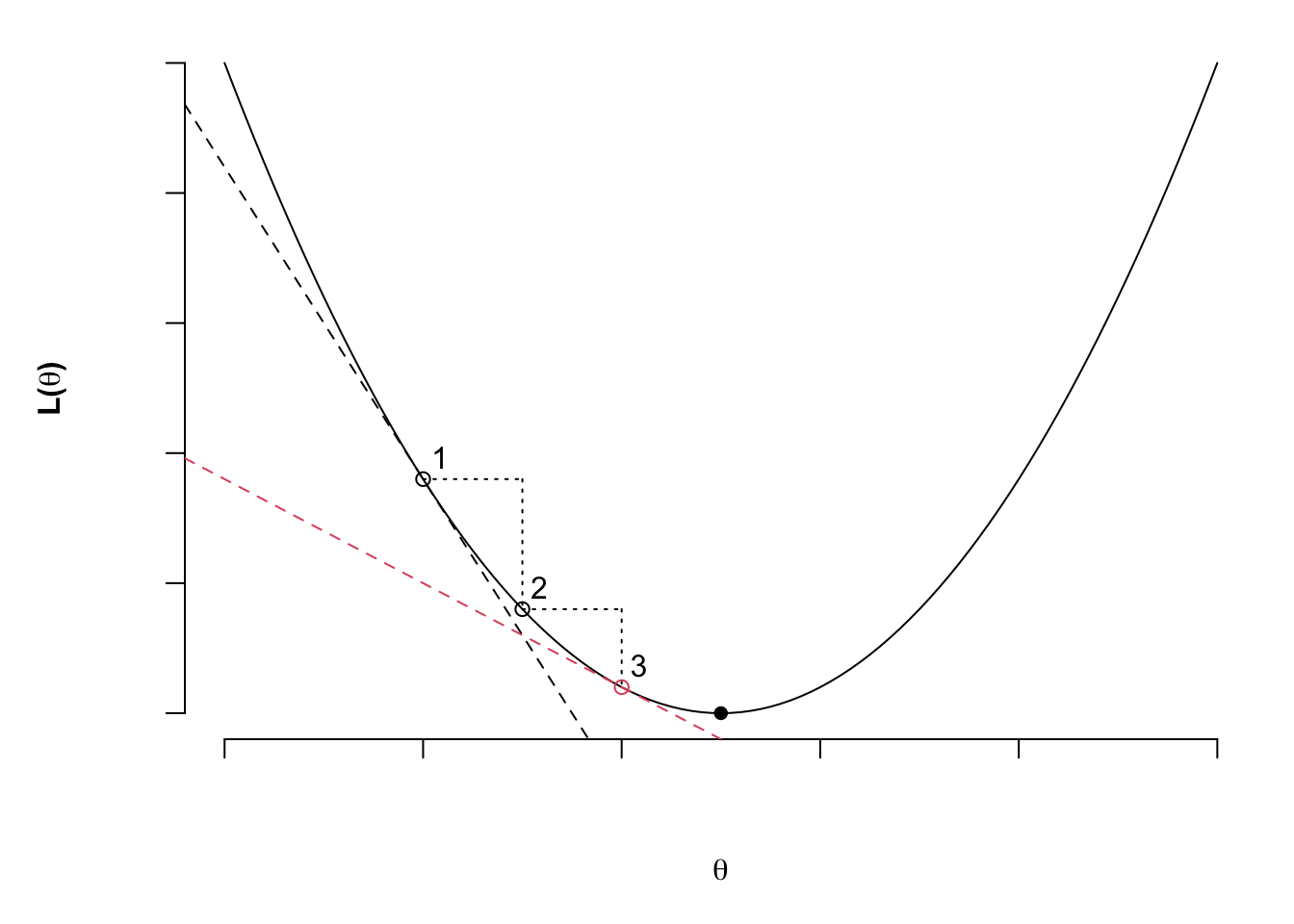
We assume the objective function is convex over the parameter space, so that we can use the partial derivatives of the objective function to estimate the values of $\boldsymbol{\theta}$. A function composed of non decreasing convex functions will be convex, see apossible weakness here.
The method is illustrated in the figure below, and is briefly as follows. The gradient of the objective function for a set of parameters values (location 1), summarised as $\boldsymbol{\hat\theta}_1$ is found, these values are used to make a further estimate $\boldsymbol{\hat\theta}_2$ and a new gradient is found, which in turn is used to estimate new parameter values. The process is repeated until further changes yield little or no improvement in the value of $L(\boldsymbol{\hat\theta}_n)$.
Finding the gradient vector
This all builds into a gradient vector that is used to move from the initial estimate to the next.
then the differentials can be expressed as;
\begin{align} \frac{\partial L}{\partial\theta_1} &= -2\sum_{i = 1}^{n}\Big( \boldsymbol{R}(\hat\theta)\odot \boldsymbol{1} \Big), \cr \qquad &\textrm{[cone threshold]}\cr \frac{\partial L}{\partial\theta_2} &= -2\sum_{i = 1}{n}\Big( \boldsymbol{R}(\hat\theta)\odot \exp\Big(-\dfrac{time_i}{\theta_3} \Big)\Big),\cr \qquad &\textrm{[cone offset]}\cr \frac{\partial L}{\partial\theta_3} &= -2\sum_{i = 1}{n}\Big( \boldsymbol{R}(\hat\theta)\odot \dfrac{\exp\Big(-\theta_2.\dfrac{time_i}{\theta_3}.time_i \Big) }{\theta_3^2}\Big),\cr \qquad &\textrm{[cone time constant]}\cr \frac{\partial L}{\partial\theta_4} &= -2\sum_{i = 1}^{n}\Big( \boldsymbol{R}(\hat\theta)\odot \dfrac{(time_i - \theta_5)}{\big(1 + \exp(time_i - \theta_5) \big) }\Big), \cr \qquad &\textrm{[S2, rod rate of recovery]}\cr \frac{\partial L}{\partial\theta_5} &= -2\sum_{i = 1}^{n}\Big( \boldsymbol{R}(\hat\theta)\odot \Big(\dfrac{\theta_4}{1+\exp(time_i - \theta_5)}- \theta_4. \exp(time_i - \theta_5)\dfrac{(time_i - \theta_5)}{(1 + \exp(time_i - \theta_5))^2} \Big)\Big). \cr \qquad &\textrm{[cone-rod break point]}\cr \end{align}
hence
\begin{align}
\nabla_\theta \boldsymbol{L(\theta)} &= \begin{bmatrix}
\frac{\partial L}{\partial\theta_1} \cr
\frac{\partial L}{\partial\theta_2}\cr
\frac{\partial L}{\partial\theta_3}\cr
\frac{\partial L}{\partial\theta_4} \cr
\frac{\partial L}{\partial\theta_5}
\end{bmatrix}
\end{align}
Having found the gradient vector then we do the descent thing
Plain gradient descent
\begin{equation}\label{eqn:vani}
\hat\theta_{n+1} =\hat\theta_{n} - \eta\nabla_\theta L(\hat\theta_{n})
\end{equation}
Momentum
\begin{equation} v_0 = \boldsymbol{0} \end{equation}
\begin{equation} v_n = \gamma v_{n-1} + \eta \nabla_\theta L(\hat\theta_{n}) \end{equation} \begin{equation} \hat\theta_{n+1} = \hat\theta_{n} - v_n \end{equation}
Nesterov
\begin{equation} v_n = \gamma v_{n-1} + \eta \nabla_\theta L( \hat\theta_{n} - \gamma v_{n-1} ) \end{equation} \begin{equation} \hat\theta_{n+1} = \hat\theta_{n} - v_n \end{equation}
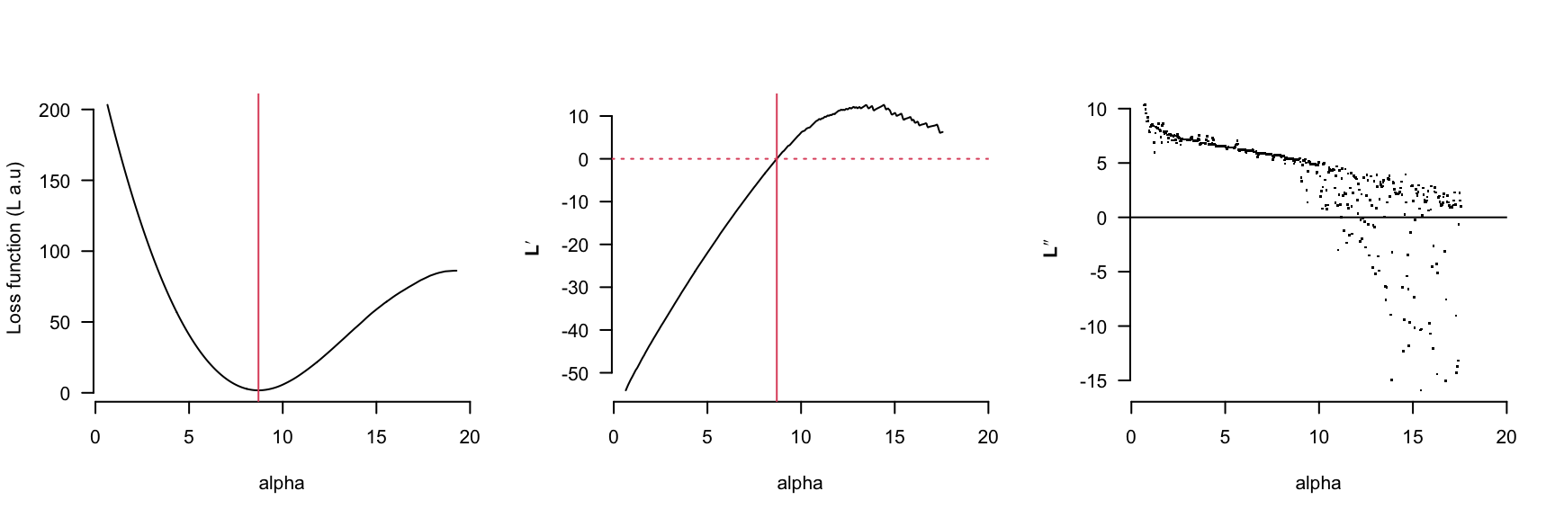
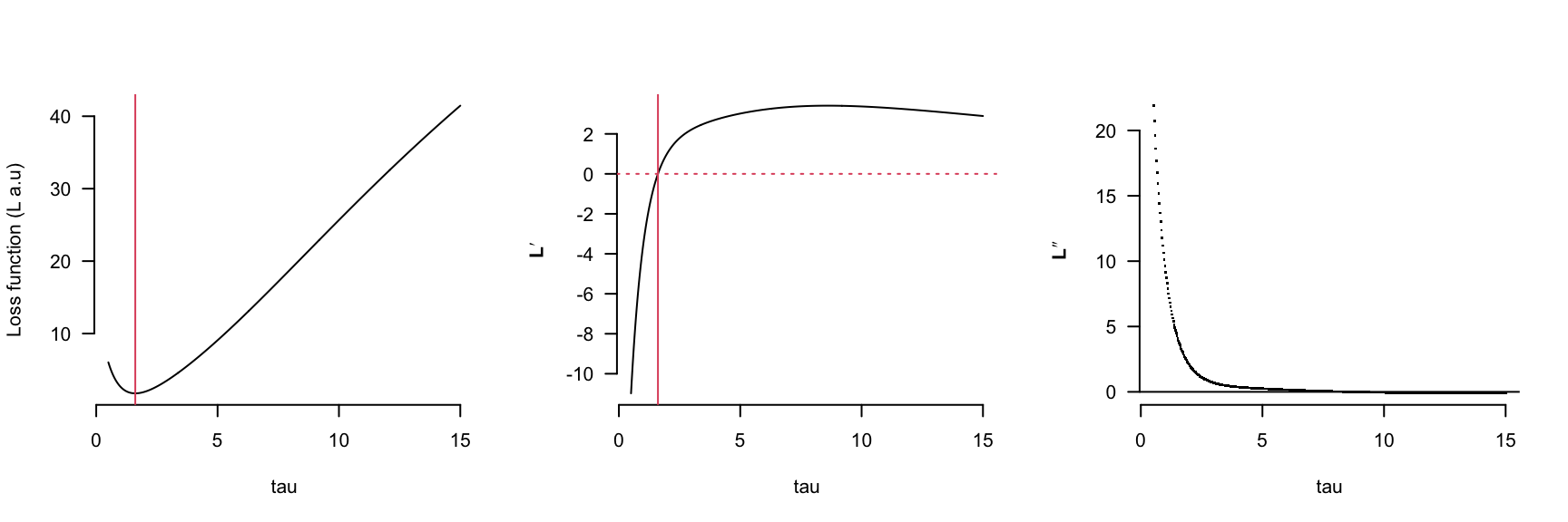
How do the gradient values vary as the estimate changes?
The first order partial differential equations are plotted below.
The parameters ct, cc and S2 are linear in the model
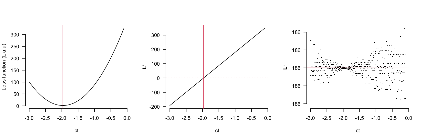
However the cone rod break time (alpha) behaves quite differently, notice that if the initial estimates for alpha and tau are greater than 12 or 6 respectively then the gradient function will direct the parameter search in the ‘wrong’ direction.
Appendix
\begin{equation} \boldsymbol{\nabla(\theta)} = \end{equation}
\begin{equation}\label{eqn:ct} \frac{\partial L}{\partial\theta_1} = \frac{\partial L}{\partial CT} = -2\sum_{i =1}^{n}{\fn{}} \end{equation}
\begin{equation}\label{eqn:cc} \frac{\partial L}{\partial\theta_2} = \frac{\partial L}{\partial CC} = -2 \sum_{i =1}^{n}\exp\Big(-\dfrac{time_i}{\theta_3} \Big).{\fn{}} \end{equation}
\begin{equation}\label{eqn:tau} \frac{\partial L}{\partial\theta_3} = \frac{\partial L}{\partial \tau} = -2\sum_{i =1}^{n}\dfrac{\exp\Big(-\dfrac{time_i}{\theta_3}\Big)\theta_2.time_i {.\fn{}}}{\theta_3^2} \end{equation}
\begin{equation}\label{eqn:s2} \frac{\partial L}{\partial\theta_4} = \frac{\partial L}{\partial{S2}} = -2\sum_{i =1}^{n}\dfrac{(time_i - \theta_5){.\fn{}}}{\big(1 + \exp(time_i - \theta_5) \big)} \end{equation}
\begin{equation}
\frac{\partial L}{\partial\theta_5} =
\frac{\partial L}{\partial \alpha} =
2\sum_{i =1}^{n}\Big(\dfrac{\theta_4}{1+\exp(time_i - \theta_5)}- \theta_4. \exp(time_i - \theta_5)\dfrac{(time_i - \theta_5)}{(1 + \exp(time_i - \theta_5))^2} \Big)
{.\fn{}}
\end{equation}